Jan Steinkühler
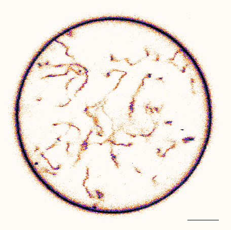
A lipid bilayer vesicle with nanotubes on the inside. Scale bar 5um.
Measuring membrane-substrate adhesion energies from the shape of adhering vesicles
When in contact with an adhesive substrate, vesicles with fluid membranes will deform to maximize the adhesion area. The balance between adhesion energy, membrane bending rigidity and vesicle volume and membrane area constraints determines the shape of the adhering vesicle. Thus measurements of the shape of an adhering vesicle can be used to approximate the membrane-substrate adhesion energy. Experimentally the method is based on fluorescence confocal imaging of adhering GUVs. Details of the method are given in the references (1,2) which should be read first. In the following the application and image analysis tools used are described. Basic knowledge of MATLAB and ImageJ is assumed. I used a semi-automated approach to extract the membrane contour instead of a completely automated contour detection. While latter might be preferred, the used approach turned out to be quite effective for a typical measurement of a few 10’s of vesicles per condition.
Note: The imaging quality and resolution will determine the precision of the method and should be optimized first. It is advantageous to use a high NA water immersion objective to achieve high resolution and limit spherical aberrations. Because the adhering vesicle shapes considered must have rotational symmetry, it is sufficient to acquire a side view of a adhering vesicle. This is conveniently done with the fast “Galvo z-stage” which allows to acquire a (x,z) image with a single confocal scan. As will become clear further below it is quite advantageous to overlay the image with the location of the adhesive substrate. This can be done elegantly by visualizing the light reflected form the water-substrate interface. On Leica SP microscopes this is accomplished using the “Reflection” presetting. Check your specific microscope setup on how to acquire such an image. This short manual assumes that you have acquired an image similar to the one shown in Fig. 1A.
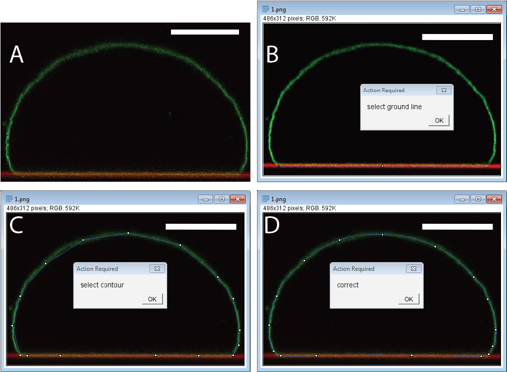
Figure 1.Confocal image (side-view) of an adhering vesicle. Membrane (green) and substrate (red).
Steps to measure adhesion energy
- The first step is to load your image into ImageJ or Fiji and load the macro provided below. After downloading into the appropriate folder of your Imagej copy, you can find the macro using Plugin -> Macros in Imagej/Fiji.
- After starting, the macro will ask you to “select the ground line” (Fig. 1B). This line is used to determine the adhesion area and the extracted adhesion energy can be quite sensitive to the precise value of adhesion area. Thus be consistent as what to count as the adhesion zone. In the overlay image of substrate and membrane signal the overlap can determined quite well by eye as the yellow region, but you might consider to use a more quantitative approach for this measure. For example you could calculate the co-localization of the two channels. This should improve the scatter of the data greatly.
- After clicking ok, the macro selects the polygon tool which you use to roughly select the membrane contour as shown in Fig 1C.
- In the next step a smooth spline is fitted through your points. Now is the time to correct the location of the points to accurately represent the membrane contour like shown in Fig 1D. Make sure to select the points such that the adhesion segement is a flat segment of the contour.
- The script will store the coordinates of the contour and adhesion disc in a file named after the image file. Note that the original image file is overwritten with the contour overlayed. The script will then open the next image file in the current directory and you can repeat steps 2-6 for each of your images. In the following the textfile with the coordinates for a particular image is called
1.txt. The coordinates are [x,y] pairs of points along the contour with the coordinates for the groundline in the first two rows. - Now start MATLAB and make sure that you download
getRV.m,tordeux_adhesive.mandangle_volume.m(links below) and all files are in the same path. Now you can calculate the area, volume and reduced volume from this contour. CallgetRV(data,scale)with the datafile andscalethe pixelsize in units of 1/µm. Note: Make sure that “importdata” imports the data as a n x 2 double. Maybe you need to look in the importdata struct for it.>> data=importdata("1.txt"); >> [rv,avg,dev,discarea]=getRV(data,7.2) rv = 0.8425 0.8424 avg = 1.0e+04 * 1.0164 8.1191 0.8425 dev = 1.0e+03 * 0.3614 4.3248 0.0001 discarea = 2.7559e+036. Each image is divided along the midpoint of the “ground line” selected in Fiji in Step 2. Thus for each image you get two values for vesicle area and volume. Here
rvis the reduced volume,avg[1]is the average area from the two mirror images,avg[2]the corresponding vesicle volume and average reduced volumeavg[3]. As a rule of thumb the corresponding standard deviations indevshould be a at least a factor of 10 smaller then the average values.discareais the total adhesion area calculated from the “Ground line”. The adhesion energy is calculated from these values:>> tordeux_adhesive(rv,avg,dev,discarea) ans = 0.4467 - The result is the adhesion energy divided by the bending rigidity kappa in units of µm^(-2). I recommend to first obtain a series of images of the same vesicle and calculate the adhesion energies for this individual vesicle. This will give you a feeling for the scatter in the calculated quantities.
If you found the analysis useful, please cite the corresponding articles.
References
- Modulating Vesicle Adhesion by Electric Fields, J. Steinkühler, J. Agudo-Canalejo, R. Lipowsky, R. Dimova Biophysical Journal 111 (7), 1454-1464, 2016 Full Text
- Analytical characterization of adhering vesicles, Tordeux, C., J-B. Fournier, and P. Galatola Physical Review E 65.4 041912, 2002
- getRV.m
- tordeux_adhesive.m
- angle_volume.m
- ImageJ Macro